Model Verification - Guiding Principles

Stan Benjamin - 2015, updated Nov 2016, Feb 2017, 2023 (in intro), 2025 (a few small changes)

The original Google Doc format is available here

• Why verify weather models?

• Key verification areas (in order of importance) for different scales/models: (details further below on how best to use each verification area)

Introduction¶

Verification can be used to assess forecast accuracy and to compare between different versions of forecast models.

Behind verification, there must be a hypothesis: A proposed innovation (model component? Data assimilation variation?) produces equal or improved forecast accuracy than a previous treatment (the control). The hypothesis should include the changes to how representation of physical processes (for model) should modify verification scores.

This hypothesis may be supported or rejected using verification - Do verification results agree with what was hypothesized? Before using statistical verification to examine an experiment, a case study should be conducted to also examine the same hypothesis - do the spatial and temporal patterns of experiment results support the hypothesis?

Verification for models is usually best applied with well-designed controlled experiments with isolatable changes. Of course, experiments need to eventually be conducted for a combined set of many changes. But these combined-change experiments cannot give good scientific answers on cause-and-effect. There should be hypotheses given for combined-change experiments based on results already available from a set of more tightly controlled experiments regarding the individual components contributing to the combined change.

Results from a variety of different verification assessment measures (vs. different kinds of observations: e.g., upper-air, surface, radiation, precipitation) for a given pair of experiments must be intercompared to look for consistency to draw a conclusion. Use of a single measure without these intercomparisons can often lead to an incorrect assessment. Examples of needed verification combinations are shown below.

Key verification consistency principles¶

• What is your hypothesis in verifying experiments?

• Look at verification against multiple observational datasets. Do they give consistent results? (e.g., compare results including biases using surface obs, upper-air (both raobs and aircraft especially for RH) and cloud/radiation obs (e.g., SURFRAD). Are results consistent also with precipitation verification vs. radar reflectivity (if appropriate)) If different experiments with different model or assimilation configurations are being compared, are results from each of these comparisons consistent with the physical hypotheses?

• Are time-series verification results consistent with time-averaged results? Inspection of time-series verification is essential to investigate a hypothesis and is also essential to ensure that the model and observation datasets do not have extreme outliers contaminating the results.

• Results should be consistent for verification against gridded data sets and especially against direct observations. (Gridded data sets, while useful to some extent, are not independent from physics-related biases in the models with which data assimilation was performed to produce those analyzed gridded data sets..)

• Check with verification results over different seasons and times of day. Verification results for a pair of experiments must also be examined for different geographical regions.

• Are the verification differences statistically significant?

• If your experiments are cold-start experiments (i.e., no cycled data assimilation), are the initial conditions biased (e.g., GFS with cold soil bias, no DA of surface observations)? Interpretation of your experiments will be heavily dependent on the accuracy of the initial conditions. Many cold-start experiments are so handicapped by initial condition biases to not be very useful.

• If your experiments are cycled, is the data assimilation missing any observations (including clouds or surface data or other important observation data set)?

In general, an innovation to a model/assimilation system should provide some kind of improved forecast skill in some verification area (e.g., precipitation, 2m temperature, clouds/radiation) and do no harm in other areas (e.g., upper-air). This means that innovations need to be evaluated over different geographic areas, times of day, and different seasons, and against different observing systems and pass this test: provide some benefit in at least some conditions and do no harm in other conditions. (This criterion is shared by NWS/NCEP and for other international NWP centers.)

There are 2 breakdowns below for verification principles:

• By NWP scale-dependent niche (storm-scale, regional short-range (RAP), global medium-range, subseasonal)

• By observation type (raob, aircraft, surface, cloud, precipitation)

Familiarity with both areas of principles is important for coming up with an appropriate set of verification tests to test an NWP change hypothesis.

These verification focus areas below are related to key phenomena addressed by different model niches. (GSL model verification webpage (Model Analysis Tool Suite) - gsl.noaa.gov/mats )

Verification Tips by Model¶

Regional/RAP-scale¶

Upper-air¶

Upper-air verification shows dynamics/physics “backbone” accuracy

1. RMS error is generally more important than bias, although bias for temp and RH at 00z or 12z (but not together) can be revealing especially for accuracy of boundary-layer processes. Biases can also indicate possible issues with radiation or cumulus or aerosols or momentum mixing aloft or gravity-wave drag.

   1. Bias - temperature and RH (better, relative at different levels. Mixing ratio not helpful with exponential behavior.)

      1. Look at by time of day - 12z vs. 00z - do not combine.

      2. Use both raobs (2x/day) and aircraft (at all times of day, at least over certain areas like US)

   2. Use 3 sources

      1. In situ obs - raobs and aircraft

      2. Gridded data - e.g. GFS analyses or RAP or HRRR analyses

      3. If results from all observations (raob, aircraft, grids) give approximately the same answer, then the result is more certain. (question - can we look at significance with multiple obs)

   3. NOTE: Recent research by Stan Benjamin and Dave Turner have revealed that raobs appear to have a low RH bias. RH bias should also be assessed using aircraft (AMDAR) observations.

Surface¶

Reveals physics accuracy, esp. over eastern US, where there is limited non-physical contamination by better agreement in elevation between surface observations and surface elevation in models

1. 2m temp/dewpoint and especially, bias, are most important due to their impact on convective environment.

   1. Note: These variables are sensitive to the diagnostic method used. It turns out that the linearly interpolated 2-m dewpoint (used unfortunately in RRFSv1) gave an unrepresentative value compared to the usually used flux-based diagnostic (used in HRRR, RAP, RUC).

2. 10m wind is not as important as 2m T/Td, although a high wind speed bias at night can be (not necessarily) related to a warm bias.

Clouds¶

Reveals physics accuracy, also post-processing and DA effects

1. Ceiling

   1. Is model geographical coverage and even cloud base level correct for CSI and bias values? Look at HSS (more appropriate for rare events and for penalty for high bias than TSS.)

   2. Use event contingency verification, not mean or RMS error in ceiling height (which gives too much effect from errors in mid- or high-level cloud less relevant to transportation).

   3. Critical for aviation users (IFR/MVFR/VFR levels are important for aviation activities), but revealing for PBL behavior. Deficient or excessive cloud coverage will lead to (or are at least associated with) boundary-layer temp/RH biases.

2. GOES-GCIP cloud coverage

   1. Is model mean cloudiness correct? Is there an under- or overforecast?

3. SURFRAD/SOLRAD - downward shortwave radiation

   1. Is model mean downward shortwave radiation reaching surface correct?

   2. Is model clear-air downward SW radiation correct?

   3. Is mean absolute error for downward SW rad more accurate?

   4. Are there geographical variations in downward SW forecast accuracy?

Precipitation¶

1. Best treated by event-based contingency verification at different precipitation thresholds.

2. 0-1h precipitation accuracy is of special importance, since the evolution of land-surface fields depends critically on this first hour of precipitation for the hourly updated models (e.g., HRRR, RRFS, RAP, RUC).

HRRR - storm-scale¶

1. Radar data (especially in warm-season)

   1. Reflectivity - CSI with obs/model scale averaged up to 20km or 40km, bias without upscaling

   2. (secondary - from radial wind) - updraft helicity tracks

2. Surface (biases, in particular, are critical for assessing accuracy of storm/cloud/precip environment. Year-round)

3. Upper-air (Are the dynamics/larger-scale fields, also important for storm prediction, accurate in the HRRR or other convection-allowing model? Also year-round)

4. Clouds (Downward shortwave radiation, ceiling)

5. Precipitation Look at bias in different thresholds.

Global¶

1. Upper-air - rawinsonde

   1. vertical profile of RMS/bias for wind, RH, temp

   2. scorecard levels - 250hPa, 850hPa, 850-100 hPa average

2. Anomaly correlation coefficient - 500 hPa heights - a close second place

3. Surface (a distant third place)

4. Clouds

   1. Simulated visible + IR imagery (as from SOS) can give good qualitative validation

   2. CERES

5. Precipitation

Subseasonal¶

Useful to evaluate the same physics suite used for regional or short-medium range NWP but evaluation here within a coupled global model

1. Precipitation - anomalies

2. MJO predictability

3. 2m temperature

4. 500h behavior - blocking frequency, mean heights, etc.

5. Stratospheric warming events

Hints for all verification¶

• Always inspect time series along with time-averaged statistics to ensure there are no outlier events from some non-model glitch value in the database.

  • If you find such an event, write to someone in Model Assessment section to possibly remove that event (if they agree) (mats.gsl@noaa.gov)

• Inspect the number of observations. Are they as expected? Look at a time series of the number of observations.

• Future: Look at the number of poor-skill cases and see if the number of poor-skill cases is reduced with a given model/assimilation change. Forecast skill is obscured by the majority of cases with high forecast skill. The true potential value of a change should be better identified by seeing if it reduces the number of bust forecasts.

  • Another way to do this is to use normal stats but stratify the events by higher error cases.

Verification Tips by Observation Type¶

Upper-air / raob verification¶

• vertical profile

• RMS errors

  • Always show model difference by checking the plot option - much easier to quickly see overall difference and magnitude of difference.

  • Times of day (00z and 12z) can generally be combined - there is usually little diurnal variation of RMS errors. (There may be unusual circumstances in which to take a look, especially if time series plots show an unexpected diurnal variation.)

• Event matching

  • Be sure to turn this on.

• Bias

  • Stratify these scores between 12z and 00z by selecting one at a time.

    • Biases can cancel out between those 00z and 12z times. Physics-related biases may have very different effect at 12z (end of night-time inversion in N. America) vs. 00z (end of daytime period with full mixing in N. America)

  • Beware of misleading statistics for high-elevation areas.

    • Reduction to isobaric levels below surface elevation may result in non-physical biases, primarily for temperature.

    • Low-level temperature biases are better examined in the eastern US or over the full CONUS area.

  • Usually better to not click on difference for bias since bias vertical profile is more easily read without difference.

• Use isobaric grid option for comparing GSD models to NCEP models

  • e.g., use FIM_prs vs. GFS instead of FIM vs. GFS

  • NCEP models (GFS, NAM) output isobaric grids only, and that is what is used in our EMB verification for those. There is more “detail” (noise) in native-level output. To use the native-level data from an EMB model will give higher error. (See below. One exception: Temperature near ground, where native data verifies better against raob data.)

  

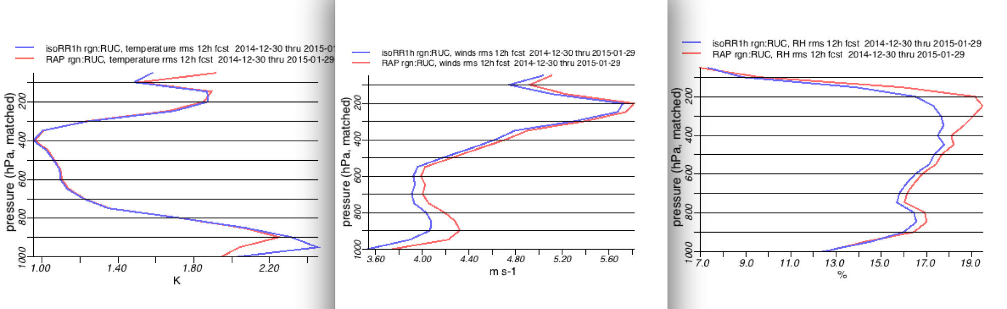
• RH

  • Given increased inaccuracy for RH measurements at temps below -30C due to very small water vapor mixing ratios, we have traditionally given much less attention to RH errors for pressure < 400 hPa than for those for p >= 400 hPa.

Surface verification¶

• Bias

  • Eastern US is generally more meaningful than western US since eastern US is less subject to elevation-reduction uncertainties, especially for 13km grids but even for 3km resolution.

  • For HRRR, both western US and eastern US stats are equally revealing.

  • Use time series of bias at a single time of day (e.g., 12h forecasts valid at 00z as representative of daytime bias)

• Variables to look - 2m temperature, 2m dewpoint, 10m wind

  • Added in late 2016 - 10m wind gust

• Diurnal

  • This is a very revealing option to see the diurnal variation of RMS or bias errors for a given forecast duration of a given model -- recommended.

Aircraft¶

• Advantage

  • Can see upper-air verification statistics for every hour, not just every 12h as for raobs.

  • unique for round-the-clock aloft skill for hourly updated models (e.g., HRRR, RAP, RUC) - only aircraft can do this.

  • Available for wind, temperature and RH.

• Caution:

  • Aircraft obs are not available in a geographical uniform distribution, especially for night-time (minimum 06-08z over US) when available primarily for package-carrier flights.

• Compare descent vs. ascent vs. enroute. Also do time series, as with any verification. Look for consistency and if it’s not there, results are probably misleading and partially incorrect.

Clouds¶

• Ceiling

  • To check if the model geographical coverage and even cloud base level correct for CSI and bias values?

  • Use CSI and bias.

    • bias might be acceptable up to 150% but 250% is definitely too much

• GOES-GCIP cloud coverage

  • To check if model mean cloudiness correct?

• SURFRAD

  • Is model mean shortwave radiation reaching surface correct?

  • Can we stratify this verification by clear vs. cloudy conditions?

• All-sky camera

  • can be used for both analyses and shert-term forecasts

• Simulated cloud albedo (visible) imagery can give good qualitative validation

• Depending on accuracy tolerances and methods used, the simulated 11 micron IR imagery can be used for quantitative verification. We have been trying this out in LAPS.

Reflectivity¶

• Resolution upscaling

  • Necessary up to 20km or 40km for CSI to capture neighborhood accuracy. Failure to do so will give misleading results that are basically reflecting bias and overforecasting of reflectivity coverage. Upscaling can be done directly before calculating event-based scores (e.g., CSI, PODy, etc.) Fractional Skill Score (Roberts and Lean 2009) also captures this scale dependency.

  • Full (3km) is effective for non-geographic assessment of model bias, i.e., too much or too little convection in model vs. observations.

Precipitation (against gridded QPE)¶

• Resolution upscaling

  • critical up to 20km or 40km or 80km for CSI, for the same reasons as for reflectivity.

Precipitation - by stations or SYNOPs¶

• Subject to geographic bias due to uneven station spacing - caveat emptor.

Anomaly correlation¶

• % of days for which AC exceeds 0.8 or 0.6 -- will automatically trend out to longer days

• AC frequency distribution

  • allows better look in % of dropout cases

• Geographical coverage:

  • Helpful to look at both NH and SH. Do not look at global AC - NH and SH results may cancel each other out.

  • Arctic and Antarctic breakdown less important but still interesting. Example: https://docs.google.com/a/noaa.gov/document/d/1CNqPAYHy0XYNkAqT5CWEz-R8X4vLiGLv1evgSVb0HLk/edit#bookmark=id.hhwkx62dmno

  • PNA - Pacific/ North America - often used by NCEP and available in Fanglin Yang’s (EMC) verification capability but not (yet) in GSD/MDB/ADB global verification

• Time period for testing global NWP model experiments

  • One-month minimum but 1 year is preferable.

  • There are seasonal variations that should be addressed.

• Truth definition:

  • Generally, we use GFS analyses but note that that gives an advantage to the GFS model for scores since its analyses and models are correlated.

  • ECMWF analyses are an option also, as done by Fanglin Yang at NCEP:

    • http://www.emc.ncep.noaa.gov/gmb/wx24fy/fimy/

    • GFS analysis verification for same period: http://www.emc.ncep.noaa.gov/gmb/wx24fy/fim/

Other observation datasets that can be used for verification¶

• Flux measurements

  • Limitation: Will be closely related to the local land surface underneath the flux measurement. That ~1.5m-wide area may well not be representative with even a HRRR grid point with a 3000m-wide area.

• Soil measurements

  • Limitation: Same as for flux measurements.

Technical Considerations¶

Also behind proposed model/assimilation changes and related verification are these issues:

• Computational efficiency. Adding expensive new capabilities need to show adequate benefit for the additional cost.

• Robust results. The new innovation should not result in crashes.

Examples of misunderstood verification¶

• Surface verification between 2 versions of the HRRR model.

  • Showed major difference

  • Inspection of the number of observations used for each model was different (by a factor of 2). (In this case, it was due to different land-use datasets used by the 2 versions of the HRRR model, but in other cases,

  • Conclusions: Inspect data from every perspective possible.

    • The verification code was well-designed to even allow inspection of the # of obs used by each model.

    • The initial assessment of an important difference was withdrawn, avoiding wasting time chasing it down.

• Differences in upper-air verification between versions of the RAP model against raobs.

  • Inspection of a time series showed that a few observations over a multi-month period (and therefore, observation-model differences) were extremely large, strongly tilting the results.

• Upper-air biases or errors vs. rawinsondes

  • The number of stations grows much smaller near 1000 hPa since most ra

References¶

• MATS article - Turner et al 2020.

  • Turner et al. (2020)

  • NOAA IR Link

• DownSW article - Benjamin et al 2025, MWR

  • Benjamin et al. (2025)

• Editorial: Forecast verification methods across time and space scales – Part I

  • December 2018, Meteorologische Zeitschrift 27(6):433-434

  • DOI: 10.1127/metz/2018/0955

  • Dorninger et al. (2018)