Contingency-table based statistical significance calculations in our Vx.

By: Bill Moninger

To address this question I talked with several statisticians, including Tom Hamill and Michael Scheuerer of PSD. They suggested I use a bootstrap/permutation approach described in Hamill (1999) (DOI: 10.1175/1520-0434(1999)014<0155:HTFENP>2.0.CO;2).

I implemented Tom’s method to get the 95% confidence levels on the statistical differences between the two models. I also discussed with Tom and Michael the issue of autocorrelation between the hourly/daily/weekly statistics for each model. Our conclusion (we looked at CSI) was this: although the CSI’s for each model exhibit considerable temporal autocorrelation and therefore non-independence, the CSI differences do not. So if we want to look at the significance of the differences, we do not need to account for serial correlation.

In order for Tom’s permutation approach to work quickly enough to work in our vx. system and in MATS, I implemented it in C-code, which turned out to be about a hundred times faster than my previous implementation in Python. (A more experienced programmer could have made more efficient Python code, but it would not likely be faster than C.)

Details of the current implementation, for use when we implement this in MATS, are way below. But first, here is information about how to run the current working implementation.

Go to the legacy (Java) code at https://ruc.noaa.gov/stats/precip_mesonets/beta/?debug=true. You probably won’t be able to run this in your browser (although it does work in Win10, with Internet Explorer 11). If you can’t run it in your browser, try the stand-alone java code at https://ruc.noaa.gov/stats/precip_mesonets/beta/GSD.PCP_MESO.jnlp.

On Mac’s, you may not be able to download and run this. In that case you can install the CheerpJ Applet Runner extension for the Chrome Browser, and then reload the page in Chrome https://ruc.noaa.gov/stats/precip_mesonets/beta/. Once you do this, you can click on the CheerpJ icon in the upper right, and select ‘Run Applets’. That will enable you to run java applets without the use of any java in Chrome. The display will take 1-3 MINUTES to start initially; after the first time it will start up faster. You’ll have to say ‘yes’ to a warning dialog that will initially come up saying the extension could “read and change data on ....noaa.gov” (meaning locally, in your browser) in order to display the data.

If you completely strike out, ask me (Bill) to make the plots you’re interested in.

You then need to choose exactly two curves to compare, and check “(show) errors” and ‘diffs: 2-1, 3-1…’. For instance,

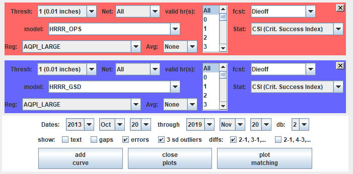
The new system only shows error bars on the difference curve. And, as before, the error bars show the 95% confidence interval. In the case above, this is the plot that results (after about 10 seconds) when you click ‘plot matching’:

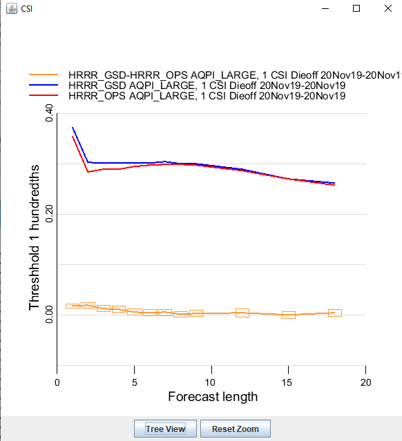
...and here’s when you get when you zoom in on the difference curve:

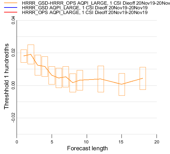
...showing that for forecast lengths < 5 hours, the differences are significant at the 95% level.

Here’s what a time series looks like:

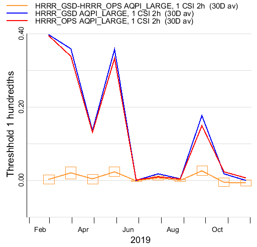
The only statistics that are available currently are CSI, Bias, Ratio, PODy, PODn, FAR, NPT, and Ntot .

Implementation details¶

Here are the details about the code that generates the error bars, mostly for Molly’s use when she implements this in MATS.

The relevant code is in /w3/emb/ruc/stats/precip_mesonets/beta/. Or, on jet (the C code only, I think) at /misc/whome/amb-verif/precip_mesonets2/permutations/

The code that generates the statistics is a combination of perl and C. The perl code (called by the java display) is getStats_file.cgi. That code generates the query for the database, which is the same for ALL statistics, and simply returns hourly contingency tables for each of two models. Here’s a sample query for the 30 day stats shown above:

NEW QUERY SET at Wed Nov 20 21:47:40 2019 using precip_mesonets2_sums database
set time_zone = '+0:00';
set group_concat_max_len = 4294967295;
select m0.valid_time as valid_time
,ceil(2592000*
floor((m0.valid_time)/2592000)+
2592000/2) as avtime
,m0.yy as hit0
,m0.yn as fa0
,m0.ny as miss0
,m0.nn as cn0,m1.yy as hit1
,m1.yn as fa1
,m1.ny as miss1
,m1.nn as cn1
from HRRR_OPS_AQPI_LARGE as m0,
HRRR_GSD_AQPI_LARGE as m1
where 1=1
and m0.valid_time = m1.valid_time
and m0.fcst_len = 2
and m1.fcst_len = 2
and m0.thresh = 1
and m1.thresh = 1
and m0.valid_time >= 1382227200
and m0.valid_time < 1574208000
and m1.valid_time >= 1382227200
and m1.valid_time < 1574208000
order by m0.fcst_len,m0.valid_time;
query took 2 secs

The perl code takes the result of the query and writes it to a file named <pid>.data.tmp, and passes the filename in env variable STAT_FILE to a c program called perm_file.c (and permutation_stats.c, and permutations.h) with executable perm_file.x (and a makefile to create the executable).

The STAT_FILE file includes

• <the desired stat>

• <a standard-deviation limit (which is not currently used)>

Many lines with these items on each line, separated by one or more spaces:

• Valid_time (seconds since 1/1/70)

• ‘atime’ (time for the averaging interval, either seconds since 1/1/70, or for dieoff, the forecast length)

• Hits, false alarms, misses, and correct rejections for model 1

• Ditto for model 2

The code will read the file, and then do the following for each group of valid times within an ‘atime’, as described in Hamil’s 1999 paper:

1. Calculate the overall statistic for model 1 and model 2

   1. If the statistic cannot be calculated, e.g. if the denominator is zero, set the statistic to BAD_VAL (= 2e30)

2. If there are < 10 (the current code may have a lower number - check the code) valid times in the atime, set the standard error to 32767.0. Otherwise,

3. Generate MAX_TRYS (currently 1000) model $a / b$ random permutations for the desired statistic assuming the null hypothesis (in which it shouldn’t matter whether contingency tables are drawn from model 1 or model 2).

4. Sort the permutation results by the difference in the model a/b statistics

5. Take the 0.025 and 0.975 level statistics to get the 95% confidence interval of the null hypothesis. In other words, if the null hypothesis is true, there’s a 95% chance that the difference in the model 1 and 2 statistic should be within the confidence interval specified.

6. Put out on standard out various diagnostic statements all starting with a semicolon.

7. Put out on standard output the following

   1. The statistic type

   2. The number of valid hours

   3. The atime (seconds since 1/1/70)

   4. The overall stat for model 1

   5. The overall stat for model 2

   6. The difference

   7. The standard error (the 95% confidence interval) divided by ($1.96*2$) (or 32767.0 if < 10 valid times)

   8. The min valid time in this atime (seconds since 1/1/70)

   9. The max valid time in this atime (seconds since 1/1/70)

Here’s the output from perm_file.x:

;stat_type from input is CSI
;sd limit from input is 0.000000
CSI 5848 1 0.414023 0.392676 -0.021347 0.001940 1549623600 1577833200
CSI 5826 2 0.353350 0.328604 -0.024747 0.002369 1549623600 1577833200
CSI 4978 3 0.342411 0.322622 -0.019788 0.002981 1549623600 1577833200
CSI 4923 4 0.339301 0.321385 -0.017916 0.002790 1549623600 1577833200
CSI 4897 5 0.336507 0.324494 -0.012013 0.002734 1549623600 1577833200
CSI 4904 6 0.334838 0.323952 -0.010886 0.002756 1549623600 1577833200
CSI 4890 7 0.335692 0.330605 -0.005087 0.003009 1549623600 1577833200
CSI 4872 8 0.333351 0.330025 -0.003326 0.002677 1549623600 1577833200
CSI 4841 9 0.335690 0.330671 -0.005019 0.002947 1549623600 1577833200
CSI 1045 10 0.386707 0.373926 -0.012780 0.004501 1549623600 1577833200
CSI 1039 11 0.385818 0.371046 -0.014773 0.005311 1549623600 1577833200
CSI 4797 12 0.329300 0.321563 -0.007737 0.003062 1549623600 1577833200
CSI 1039 13 0.376310 0.368715 -0.007595 0.004984 1549623600 1577833200
CSI 1040 14 0.365716 0.360703 -0.005012 0.005342 1549623600 1577833200
CSI 4744 15 0.308874 0.306540 -0.002333 0.003272 1549623600 1577833200
CSI 1030 16 0.352834 0.349927 -0.002907 0.004475 1549623600 1577833200
CSI 1028 17 0.350249 0.348817 -0.001433 0.005121 1549623600 1577833200
CSI 4511 18 0.299343 0.297272 -0.002071 0.002870 1549623600 1577833200
CSI 118 22 0.399792 0.395230 -0.004562 0.007200 1549623600 1577833200
CSI 124 23 0.335956 0.340390 0.004434 0.010897 1549623600 1577833200
CSI 366 24 0.267666 0.264880 -0.002786 0.008809 1549623600 1577833200

(this executable took about 5 seconds)

The perl code then takes these results, does the standard bookkeeping (finds gaps, insufficient averaging intervals, etc), scales the data and sends it back to the java display code. (The java code treats values > 32766 as NaNs.)

To recompile the executable simply edit perm_file.c, permutation_stats.c, permutations.h , and then use the makefile by typing ‘make’ at the console. A new perm_file.x should be created by the make.

I experimented with a perm_memory.c (and perm_memory.x - see the makefile), which takes its input from standard in rather than a file, but I couldn’t get it to run reliably from perl. You might have better luck with python. perm_memory.c only differs from perm_file.c by replacing ‘stream’ with ‘stdin’ in a couple of fgets calls (and by not opening a stream to/from STAT_FILE).